Why say lot word when few do trick?

It's almost impossible to watch this Kevin clip without coming to the conclusion: he's onto something.

His abbreviated sentences do seem to convey the same information as their verbose original. Can we formalize this idea of using fewer words to say the same thing? How "few" can we go without losing information?

These questions lead to one of the most profound ideas in machine learning: the Minimum Description Length (MDL) Principle. It's so important that when Ilya Sutskever gave John Carmack a list of 30 papers and said:

If you really learn all of these, you'll know 90% of what matters today.

4 of them were on this topic 1 2 3 4.

The MDL principle fundamentally changed the way I see the world. It's a new perspective on familiar concepts like learning, information, and complexity. This blog post is a high-level, intuition-first introduction to this idea.

Strings

Let's start with this question: how complex are these binary strings?

1. $00000000000000000000$
2. $10001000100010001000$
3. $01110100110100100110$

The first one seems dead simple: just a bunch of zeros. The second is a bit more complex. The third, with no discernable pattern, is the most complex.

Here's one way to define complexity, called Kolmogorov complexity: the length of a string is the shortest program in some programming language that outputs it. Let's illustrate with Python:

1. To get $00000000000000000000$, we'd write:

def f():
    return "0" * 20

2. To get $10001000100010001000$, we need to type a bit more:

def f():
    return "1000" * 5

3. To get $01110100110100100110$, we have to type out the whole string:

def f():
    return "01110100110100100110"

Making this mathematically precise takes some work: we need to define the language, measure the length of programs in bits, etc. . But that's the basic idea: an object is complex if we need a long Python function to return it. This function is often called a description of the string, and Kolmogorov complexity the minimum description length.

What separates these strings from each other? For 1 and 2, we can exploit their repeating pattern to represent them in a more compact way; such a regularity does not exist in 3. Generally, we can think about complexity in terms of data compression:

• A string is complex if it is hard to compress.
• Given a string, the most optimal compression algorithm gives us its minimum description, whose length is its Kolmogorov complexity.

Here's a claim that I'll back up through the rest of this post: compression is actually the same thing as learning. In this example, we have learned the essence of the first string by writing it as "0" * 20. Having to spell out the third string exactly means that we haven't learned anything meaningful about it.

Points

What is the Kolmogorov complexity of these 10 points?

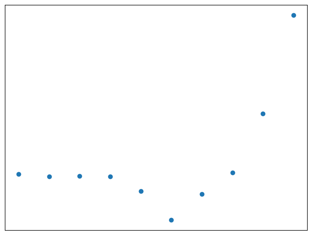
That's equivalent to asking for the minimum description length of these points. Of course, we can just describe each point by its coordinate, but can we do better?

Here's an idea: let's draw a line through the points and use it to describe each point. That means describing 2 things: the line + how the far each point is from the line.

Here are some attempts:

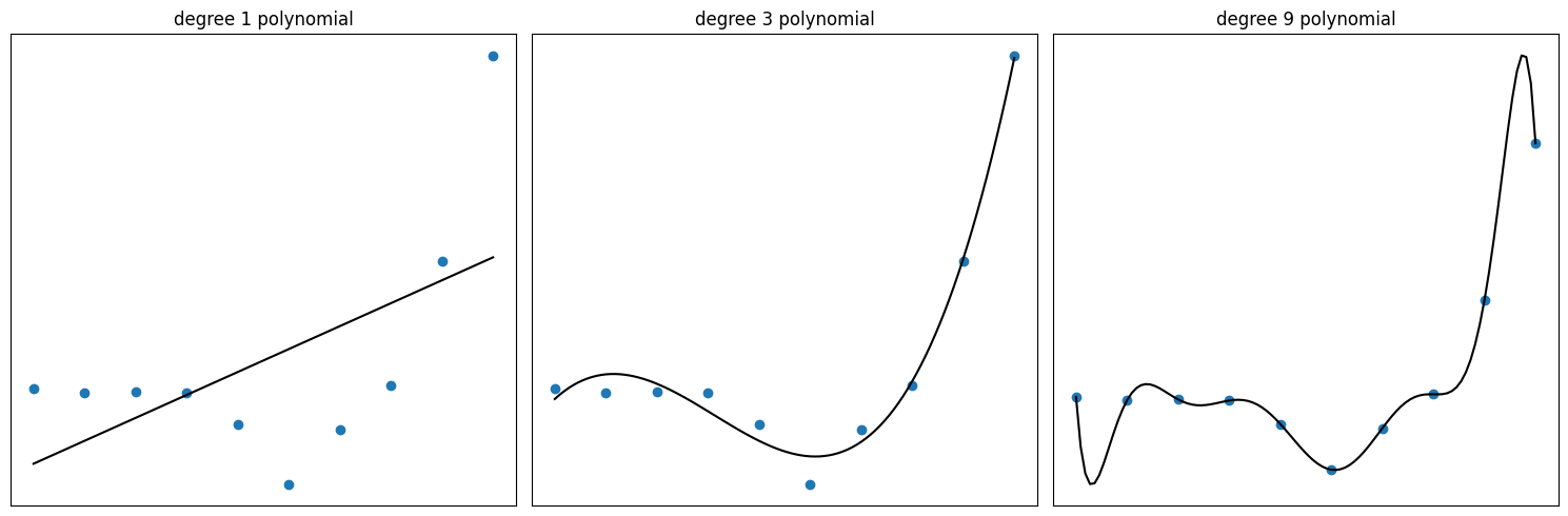
My knee-jerk reaction to these lines is: left and right bad, middle good! Under/over-fitting, bias/variance tradeoff, generalizing to unseen data, etc... But there's another way to see why the middle one is best: it gives the shortest description of these points.

The descriptions would look something like:

1. I have a line $y = 0.58x -0.12$ and it misses the first point by $0.21$, the second by $0.13$...
2. I have a line $y = 5.45x^3 - 5.68x^2 + 1.19x + 0.06$ and it misses the first point by $0.03$, the second by $-0.05$...
3. I have a line $y = -15348.64x^9 + 67461.06x^8 - 123937.33x^7 + ...$ and it fits each point perfectly.

In the first case, it's easy to describe the line, but it'll take some effort to describe how far each point is from the line, the errors. The third line is very complicated to describe, but we don't need to spend any time on the errors. The middle one strikes a balance.

More generally, we call the line a hypothesis $H$, drawn from a set $\mathcal{H}$ of hypotheses, e.g. all polynomials. There is a tradeoff between the description length $L$ of the hypothesis (the coefficients), and the description length of the data $D$ when encoded with the help of the hypothesis (the errors). We want to find an $H$ that minimizes the sum of these 2 terms:

That was all quite hand-wavy. How can we formalize the intuition that the errors of the 1st degree polynomial are "harder to describe" than those of the 3rd degree polynomial? The next section uses tools from information theory to make these calculations precise.

Coding in bits

Formally defining description length essentially boils down to encoding real numbers – coefficients, errors – in bits.

Here's a naive way to do it: type the number in Python. The float type uses 64 bits to represent every number. It represents 0, 0.1, and 1.7976931348623e+308 (the largest possible representation) using the same number of bits. That's too wasteful for our purpose of finding the minimum description: we want to encode each number in as few bits as possible.

In reality, we're far more likely to see 0 and 0.1 than 1.7976931348623e+308 (assuming the coefficients and errors come from, say, a Gaussian distribution). What if we use a shorter code for the more likely numbers like 0 and 0.1, and a longer code for the those rare events like 1.7976931348623e+308? Theoretically, the optimal code length is $-\log_2(p(x))$, where $p(x)$ is the probability of event $x$.

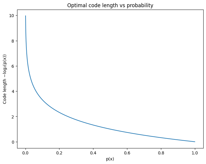
For example, if a number comes up as often as 50% of the time, you should represent it with only 1 bit.

Assuming the coefficients and errors follow a Gaussian distribution with mean $0$, we can chop up the real number line into small intervals of size $t$ and assign each interval with a discrete probability $p(x)$.

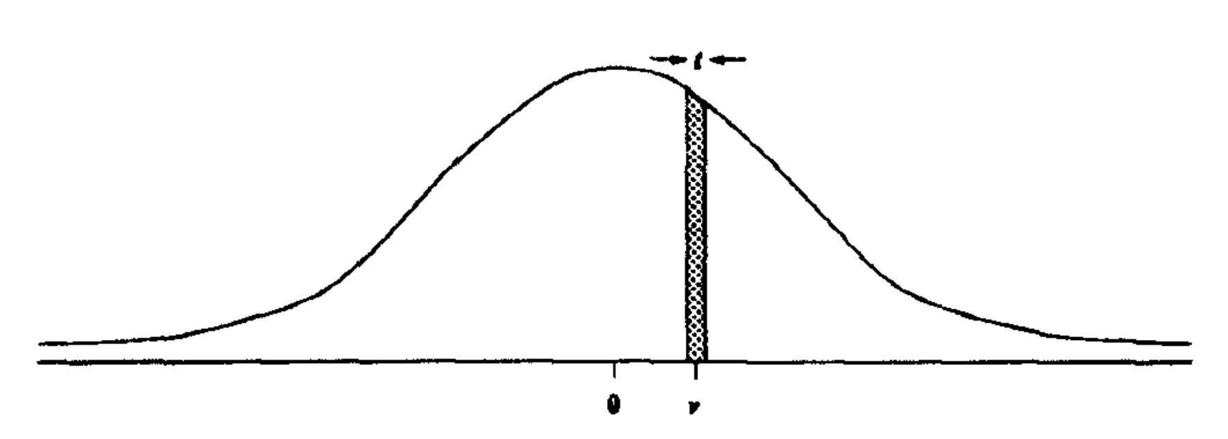
Given any real number $v$, we can discretize it by taking a small interval of size $t$ around it. For small enough $t$, can approximate the probability density at the interval with $t * g(x)$, where $g(x)$ is the Gaussian pdf with mean $0$. The picture is from sections 3 and 4 of Hinton et al. 3, which contain a detailed explanation of this method.

Given a probability, we can assume the optimal code length $-\log_2(p(x))$ and calculate the minimum number of bits needed to encode our number .

Now, we're ready to compute each term of our equation for description length:

Coding the coefficients, $L(H)$

Let's encode each of our polynomial coefficient $w_i$, starting with its discretized probability:

where $\sigma_w$, the standard deviation of the Gaussian we use, is a parameter we choose.

Calculating the optimal code length, in $\log_2 (e)$ bits (or nats):

Summing over all coefficients $w_1, ..., w_n$ to get the code length of the polynomial:

We see that minimizing the code length of the polynomial is equivalent to minimizing the term $\sum_{i=1}^n w_i^2$. In other words, we want to keep the coefficients small.

Coding the errors, $L(D|H)$

Applying the same technique to each error term $|d_c - y_c|$, where $d_c$ is the true data point and $y_c$ is our polynomial's approximation:

Here, $\sigma_d$ should be optimally set to the standard deviation of the points. Computing the full code length over the 10 data points:

Minimizing the code length of the errors is equivalent to minimizing $\sum_{c=1}^{10} (d_c - y_c)^2$, i.e. we want the errors to be small.

Regression & Learning

Adding the two terms together, we get a minimization objective $C(D)$ equivalent to minimizing the description length $L(D)$:

This fits our intuition that we want to have small coefficients that minimize the errors: the degree 3 polynomial is best.

This formula is also the minimization objective of ridge regression. We never explicitly thought about mean-squared error (MSE) or L2 regularization: they fell out of our quest for the shortest description of our data.

Under this interpretation, $\sigma_w$ is a hyperparameter of the model that lets us tweak the regularization strength. In the MDL view, its just the width of the Gaussian we used to discretize our coefficients. A small $\sigma_w$ implies a narrow coefficient distribution and, in turn, stronger regularization.

Choosing the Gaussian is reasonable and popular, though somewhat arbitrary. This is called the noise model: what distribution do we assume of our coefficients and errors? If we had chosen the Laplace distribution, we would have derived lasso regression with L1 regularization.

Back to the claim on compression being the same as learning: perhaps you can agree that these two summaries of this example are equivalent:

1. We have compressed these points using a 3rd degree polynomial, allowing us to describe them in very few bits.
2. We have learned a good model of these points, a 3rd degree polynomial, which approximates the underlying distribution.

Words

Modern LLMs like GPT are large Transformers with billions of parameters. They can also be understood through the lens of compression. Taken literally, we can use LLMs to losslessly compress text, just like gzip.

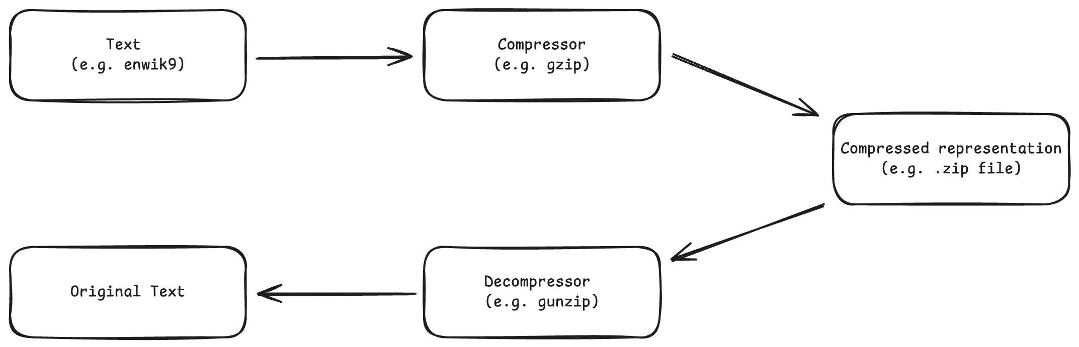
Lossless compression encodes text into a compressed format and enables recovering the original text exactly. enwik9 is the first GB of the English Wikipedia dump on Mar. 3, 2006, used in the Large Text Compression Benchmark.

Like the polynomial through the points, an LLM can be used as a guide to encode text. Instead of describing each word literally, we only need to describe "how far" it is from the LLM's predictions. I'll omit the details, but you can read more about this encoding method, called arithmetic coding, here.

Researchers found that this compression method using LLMs is far more efficient than tools like gzip 5.

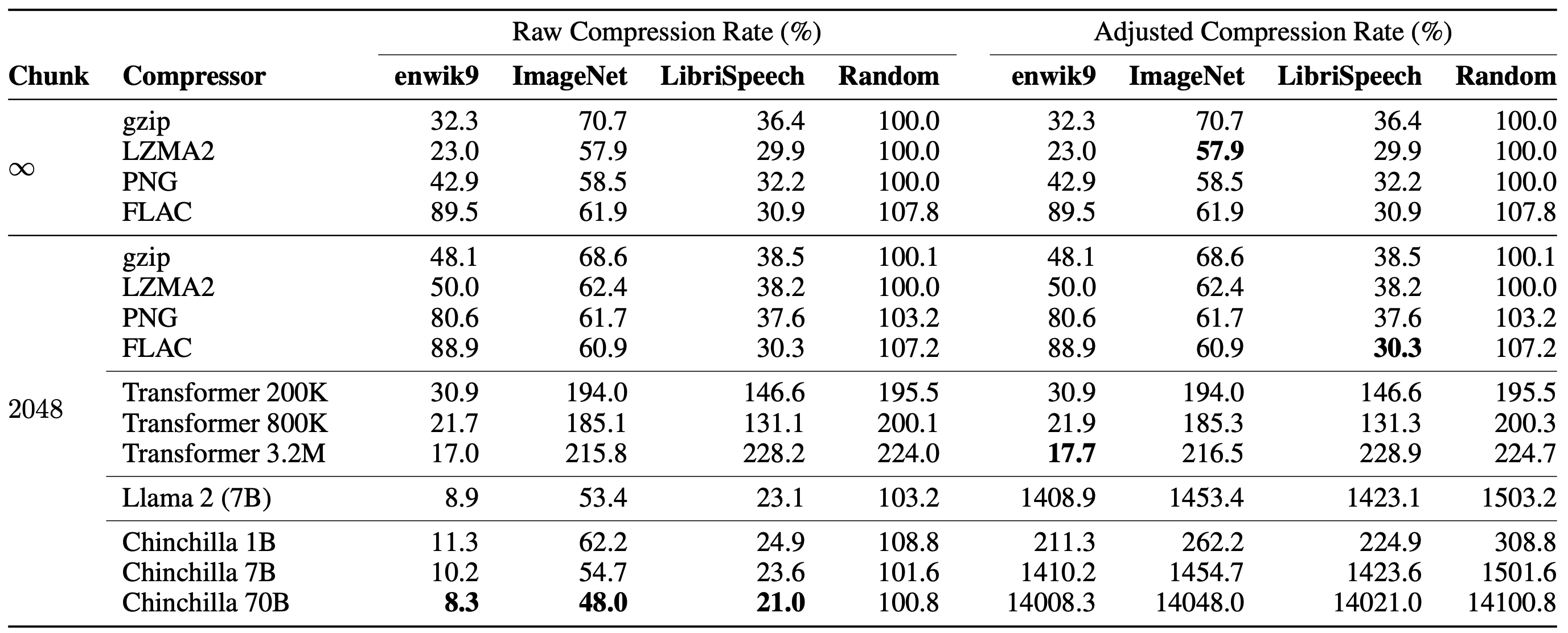
ImageNet and LibriSpeech are popular image and speech datasets. Chunk size accounts for the limited context window of LLMs, whereas gzip can operate on a much larger range and exploit more compressible patterns.

LLMs like Llama and Chinchilla managed to compress enwik9, a text file used to benchmark compression algorithm, to 10% its original size, compared to gzip's 30%. LLMs have clearly learned patterns in the text that are useful for compression.

As a crude analogy, imagine you are an expert in learning and compression. You know by heart every concept in this blog post. Reproducing this blog post just requires noting the differences between your understanding and my explanations: maybe I've phrased things differently than you would, or made a mistake. Now imagine reproducing a blog post on a topic you know nothing about or, say, in an unknown language. The latter task requires much more effort, and in the worst case, rote memorization.

More remarkably, even though Llama and Chinchilla are trained primarily on text, they are quite good at compressing image patches and audio samples, outperforming specialized algorithms like PNG. Somehow, the word patterns LLMs learn can be used to compress images and audio too. Words, images, audio: all slivers of the same underlying world.

The compression efficiency of LLMs comes at a cost: the size of their weights. This is shown on the right half of the table: "Adjusted Compression Rate". Technically, the minimum description length includes these weights in its $L(H)$ term, like how we coded the polynomial coefficients in addition to the errors. Practically, we don't want to lug around all the Llama weights every time we compress a file.

Although Llama and Chinchilla are not practical compressors––at least not until the scale of data exceeds terabytes––the authors found that training specialized transformers (Transformer 200K/800K/3.2M in the table) on enwik9 did achieve better weight-adjusted compression rate than gzip, though they don't generalize as well to other modalities.

If we try to compress all of human knowledge, as these foundation models set out to do, the $L(H)$ term will be negligible. A few GBs of model weights is nothing compared to the vastness of the internet, but they pack a whole lot. I felt this viscerally when chatting with Ollama on a flight without internet. Somehow, practically all of human knowledge is right in front of me in this inconspicuous piece of metal. That blew my mind.

Final thoughts

The MDL principle is such a profound perspective because so many powerful ideas can be cast in term of it. We saw a concrete example with linear regression. I'll close with two more.

Occam's Razor

Occam's Razor is the philosophical principle that the simplest explanation is usually the best.

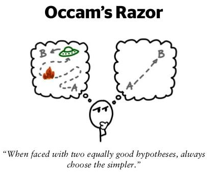
In statistical modeling, this is literally true in a mathematically precise way: the model that explains the data in the fewest number of bits is the best.

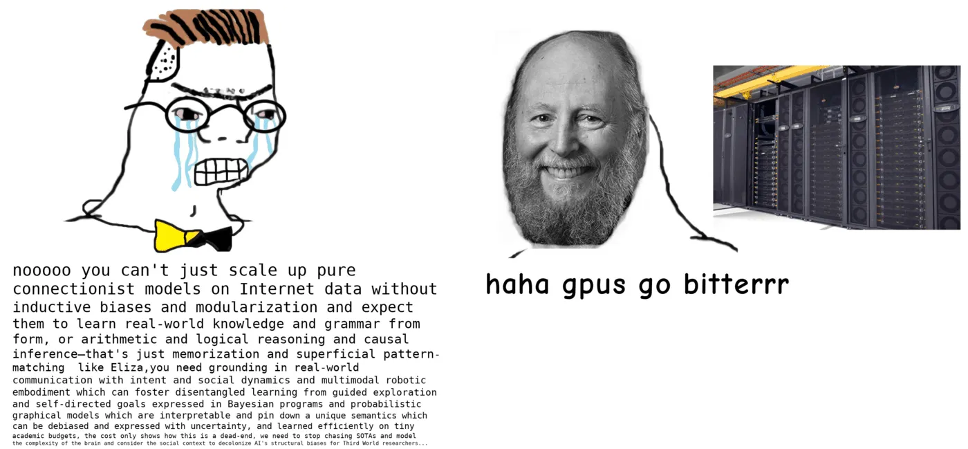
The Bitter Lesson

The Bitter Lesson in machine learning is that general methods leveraging increasing compute tends to outperform hand-crafted ones that rely on expert domain knowledge.

For example, the best chess algorithms used to encode human-discovered heuristics and strategies, only to be blown away by a "brute-force" method based only on deep search. Same story with Go. The leading algorithms are not told anything about Go beyond its rules: they discover strategies via deep learning, search, and self-play, even ones that stun the best human player in the world. This lesson has played out in many fields time and again: computer vision, NLP, even protein structure prediction.

https://danieljeffries.substack.com/p/embracing-the-bitter-lesson

The story of machine learning is one of the repeated failure of our biases, clever tricks, and desire to teach our models the world in the way we see it. From the MDL perspective, the best model of the world is the one with the minimum description. Each bias we remove is a simplification of our description. The simplest description always wins.

Acknowledgements

Thank you to Etowah Adams and Daniel Wang for reading a draft of this post and giving feedback.

References

Shen, A., Uspensky, V. A., & Vereshchagin, N. Kolmogorov Complexity and Algorithmic Randomness. Mathematical Surveys and Monographs (2017).
Grünwald, P. A tutorial introduction to the minimum description length principle. arXiv (2004).
Hinton, G. E., & van Camp, D. Keeping the neural networks simple by minimizing the description length of the weights. Proceedings of the sixth annual conference on Computational learning theory (1993).
Aaronson, S. The First Law of Complexodynamics. Shtetl-Optimized (2011).
Delétang, G., Ruoss, A., Duquenne, P. A., Catt, E., Genewein, T., Mattern, C., Grau-Moya, J., Wenliang, L. K., Aitchison, M., Orseau, L., Hutter, M., & Veness, J. Language Modeling Is Compression. arXiv (2024).
- As you can probably guess, finding the minimum program is an intractable problem in more practical situations. In fact, Kolmogorov complexity is generally not computable.
- Technically, we need an infinite number of bits because real numbers have an infinite decimal expansion. Practically, we approximate to some finite decimal point.
- In practice, we need an encoding algorithm (e.g. Huffman coding or Arithmetic coding). The codes produced by these methods are bounded by, and don't usually achieve, the theoretical optimal length .
- For classic algorithms like
gzip, the term is the length of program in its programming language, which is at most a few KBs, negligible compared to an LLM's weights.