What we can learn from evolving proteins

Proteins are remarkable molecular machines that orchestrate almost all activity in our biological world, from the budding of seed to the beating of a heart. They keep us alive, and their malfunction makes us sick. Knowing how they work is key to understanding the precise mechanisms behind our diseases – and to coming up with better ways to treat them. This post is a deep dive into some statistical methods that – through the lens of evolution – give us a glimpse into the complex world of proteins.

Amino acids make up proteins and specify their structure and function. Over millions of years, evolution has conducted a massive experiment over the space of all possible amino acid sequences: those that encode a functional protein survive; those that don't are extinct.

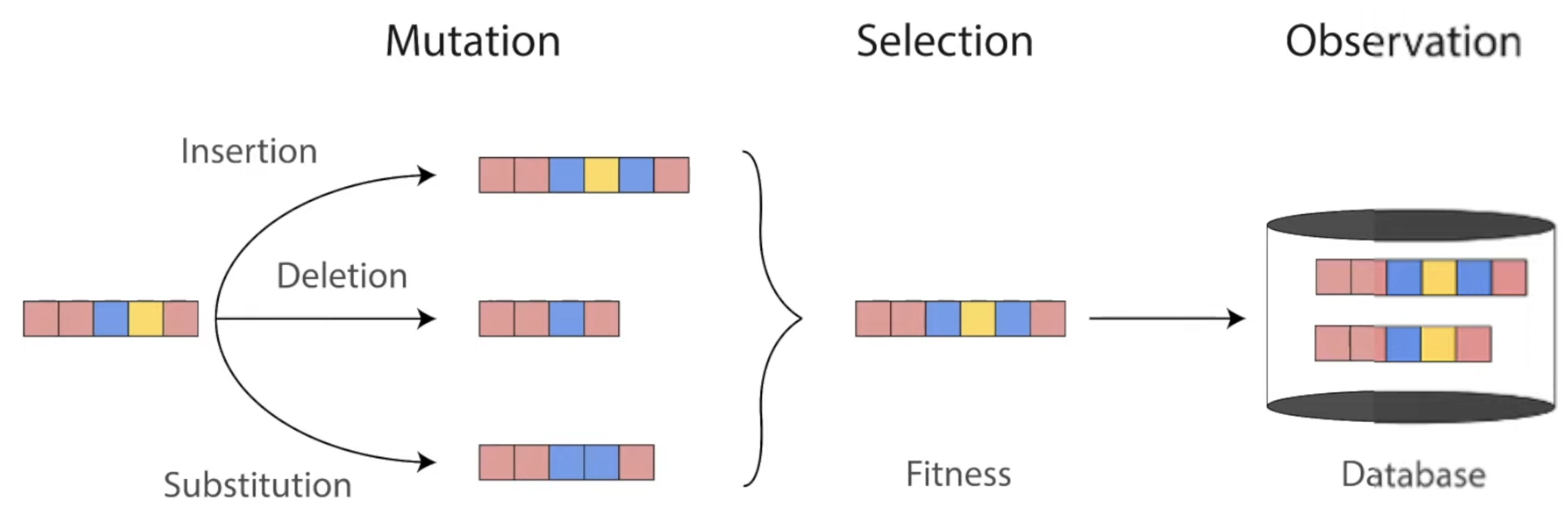
Throughout evolution, mutations change the sequences of proteins. Only the ones with highest fitness survive to be found in our world today. Diagram from Roshan Rao's awesome dissertation talk.

We can learn a surprising lot about a protein by studying similar variants of it we find in nature (its protein family). These hints from evolution have empowered breakthroughs like AlphaFold and many cutting-edge methods in predicting protein function. Let's see how.

A Multiple Sequence Alignment (MSA) compiles known variants of a protein – which can come from different organisms – and is created by searching vast protein sequence databases.

A signal hidden in MSAs: amino acid positions that tend to co-vary in the MSA tend to interact with each other in the folded structure, often via direct 3D contact. In the rest of this post, we'll make this idea concrete.

In search of a distribution

Let's start with the question: given an MSA and an amino acid sequence, what's the probability that the sequence encodes a functional protein in the family of the MSA? In other words, given a sequence $A = (A_1, A_2, ..., A_L)$, we're looking for a fitting probability distribution $P(A)$ based on the MSA.

Knowing $P$ is powerful. It lends us insight into sequences that we've never encountered before (more on this later!). Oftentimes, $P$ is called a model. For the outcome of rolling a die, we have great models; proteins, unfortunately not so much.

Counting amino acid frequencies

Let's take a closer look at the MSA:

Some positions have the same amino acid across almost all rows. For example, every sequence has L in the first position – it is evolutionarily conserved – which means that it's probably important!

To measure this, let's count the frequencies of observing each amino acid at each position. Let $f_i(A_i)$ be the frequency of observing the amino acid $A_i$ at position $i$.

If we compile these frequencies into a matrix, we get what is known as a position-specific scoring matrix (PSSM), commonly visualized as a sequence logo.

A sequence logo generated from our MSA. The height of each amino acid indicates its degree of evolutionary conservation.

Given some new sequence $A$ of $L$ amino acids, let's quantify how similar it is to the sequences in our MSA:

$E(A)$ is big when the amino acid frequencies in each position of $A$ matches the frequency patterns observed the in MSA – and small otherwise. For example, if $A$ starts with the amino acid L, then $f_1(\text{L}) = 1$ is contributed to the sum; if it starts with any other amino acid, $0$ is contributed.

$E$ is often called the energy function. It's not a probability distribution, but we can easily turn it into one by normalizing its values to sum to $1$ (let's worry about that later).

Pairwise frequencies

But what about the co-variation between pairs of positions? As hinted in the beginning, it has important implications for the structure (and hence function) of a protein. Let's also count the co-occurrence frequencies.

Let $f_{ij}(A_i, A_j)$ be the frequency of observing amino acid $A_i$ at position $i$ and amino acid $A_j$ at position $j$.

Adding these pairwise terms to our energy function:

Now, we have a simple model that accounts for single-position amino acid frequencies and pairwise co-occurrence frequencies! In practice, the pairwise terms are often a bit more sophisticated and involve some more calculations based on the co-occurrence frequencies (we'll walk through how it's done in a popular method called EVCouplings soon), but let's take a moment to appreciate this energy function in this general form.

As it turns out, physicists have studied this function since the 1950s, in a different context: the interacting spins of particles in solids like magnets. The $J_{ij}$ terms capture the energy cost of particles $i$ and $j$ coupling with each other in their respective states: its magnitude is big if they interact, small if they don't; the $h_i$ terms capture the energy cost of each particle being in its own state.

They call this the Potts model, and a fancy name for the energy function is the Hamiltonian. This fascinating field of physics applying these statistical models to explain macroscopic behaviors of matter is called statistical mechanics.

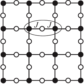
The Potts model on a square lattice. Black and white dots are in different states. Figure from https://arxiv.org/abs/1511.03031.

Global pairwise terms

Earlier, we considered using $f_{ij}$ as the term capturing pairwise interactions. $f_{ij}$ focuses on what's happening at positions $i$ and $j$ – nothing more. It's a local measurement. Imagine a case where positions $i$ and $j$ each independently interact with position $k$, though they do not directly interact with each other. With this transitive correlation between $i$ and $j$, the nearsighted $f_{ij}$ would likely overestimate the interaction between them.

To disentangle such direct and indirect correlations, we want a global measurement that accounts for all pair correlations. EVCouplings is a protein structure and function prediction tool that accomplishes this using mean-field approximation 2. The calculations are straightforward:

1. Compute the difference between the pairwise frequencies and the independent frequencies and store them in a matrix $C$, called the pair excess matrix.

2. Compute the inverse of this matrix, $C^{-1}$, the entries of which are just the negatives of the $J_{ij}$ terms we seek.

The theory behind these steps is involved and beyond our scope, but intuitively, we can think of the matrix inversion as disentangling the direct correlations from the indirect ones. This method is called Direct Coupling Analysis (DCA).

The distribution

We can turn our energy function into a probability distribution by 1) exponentiating, creating an exponential family distribution that is mathematically easy to work with, and 2) dividing by the appropriate normalization constant $Z$ to make all probabilities sum to 1.

Predicting 3D structure

Given an amino acid sequence, what is the 3D structure that it folds into? This is the protein folding problem central to biology. In 2021, researchers from DeepMind presented a groundbreaking model using deep learning, AlphaFold 8, declaring the problem as solved. The implications are profound. (Although the EVCouplings approach to the this problem we will discuss cannot compete with AlphaFold in accuracy, it is foundational to AlphaFold, which similarly relies heavily on pairwise interaction signals from MSAs.)

Myriad forces choreograph the folding of a protein. Let's simplify and focus on pairs of amino acid positions that interact strongly with each other – and hypothesize that they are in spatial contact. These predicted contacts can act as a set of constraints from which we can then derive the full 3D structure.

Hovering over the blue link, we see that positions $2$ and $8$ tend to co-vary in the MSA – and they are in contact in the folded structure. Presumably, it's important to maintaining the function of the protein that when one position changes, the other also changes in a specific way – so important that failure for a sequence to do so is a death sentence that explains its absence in the MSA. Let's quantify this co-variance.

Mutual information

Our $f_{ij}$ is a function that takes in two amino acids: $f_{ij}(A_i, A_j)$; however, we would like a direct measure of interaction given only positions $i$ and $j$, without a dependence on specific amino acids. In other words, we want to average over all possible pairs of amino acids that can inhabit the two positions $i$ and $j$. To do this in a principled and effective way, we can use a concept called mutual information:

where $\mathcal X$ is the set of 20 possible amino acids.

Mutual information measures the amount of information shared by $i$ and $j$: how much information we gain about $j$ by observing $i$. This concept comes from a beautiful branch of mathematics called information theory, initially developed by Claude Shannon at Bell Labs in application to signal transmission in telephone systems.

In our case, a large $MI_{ij}$ means that positions $i$ and $j$ are highly correlated and therefore more likely to be in 3D contact.

Direct information

As we mentioned, the local nature of $f_{ij}$ can be limiting: for one, it's bad at discerning transitive correlations that might convince us of spurious contacts. EVCouplings uses a different quantity to approximate the probability that $i$ and $j$ are in contact:

where the $J_{ij}$'s are the global interaction terms obtained by mean-field approximation, and the $\tilde{h}$ terms can be calculated by imposing the following constraints:

These constraints ensure that $P_{i j}^{D i r}$ follows the single amino acid frequencies we observe. For each pair of positions:

1. Let's fix the amino acid at position $i$ to be L. Consider $P_{i j}^{D i r}(L, \mathrm{A_j})$ for all possible $A_j$'s. If we sum them all up, we get the probability of observing $L$ independently at position $i$, which should be $f_i(L)$.

2. The same idea but summing over all $A_i$'s.

Once we have $P_{i j}^{D i r}$, we can average over all possible $A_i$'s and $A_j$'s like we did for mutual information:

This measure is called direct information, a more globally-aware measure of pairwise interactions. When compared to real contacts in experimentally determined structures, DI performed much better than MI, demonstrating the usefulness of considering the global sequence context 1.

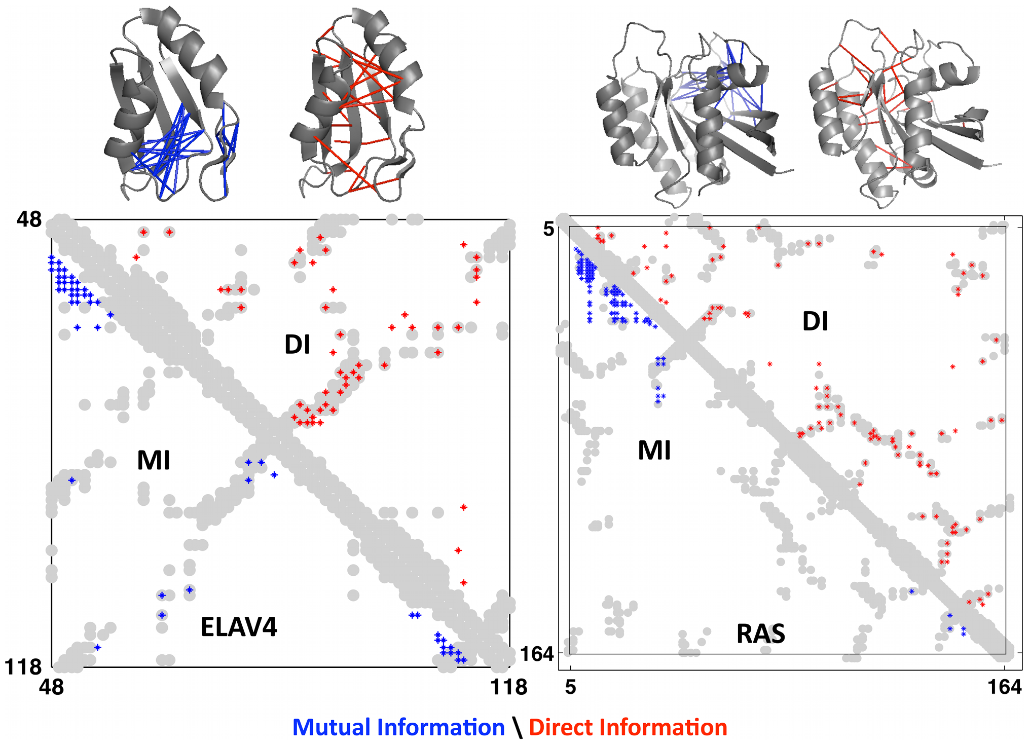
Axes are amino acid positions. The grey grooves are the actual contact in the experimentally obtained structures. The red dots are the predicted contacts using DI; the blue dots are the predicted contacts using MI. Data is shown for 2 proteins: ELAV4 and RAS. Figure from 1.

Constructing the structure

Given predicted contacts by DI, we need to carry out a few more computational steps – e.g. simulated annealing – to generate the full predicted 3D structure. Omitting those details: the results are these beautiful predicted structures that closely resemble the real structures.

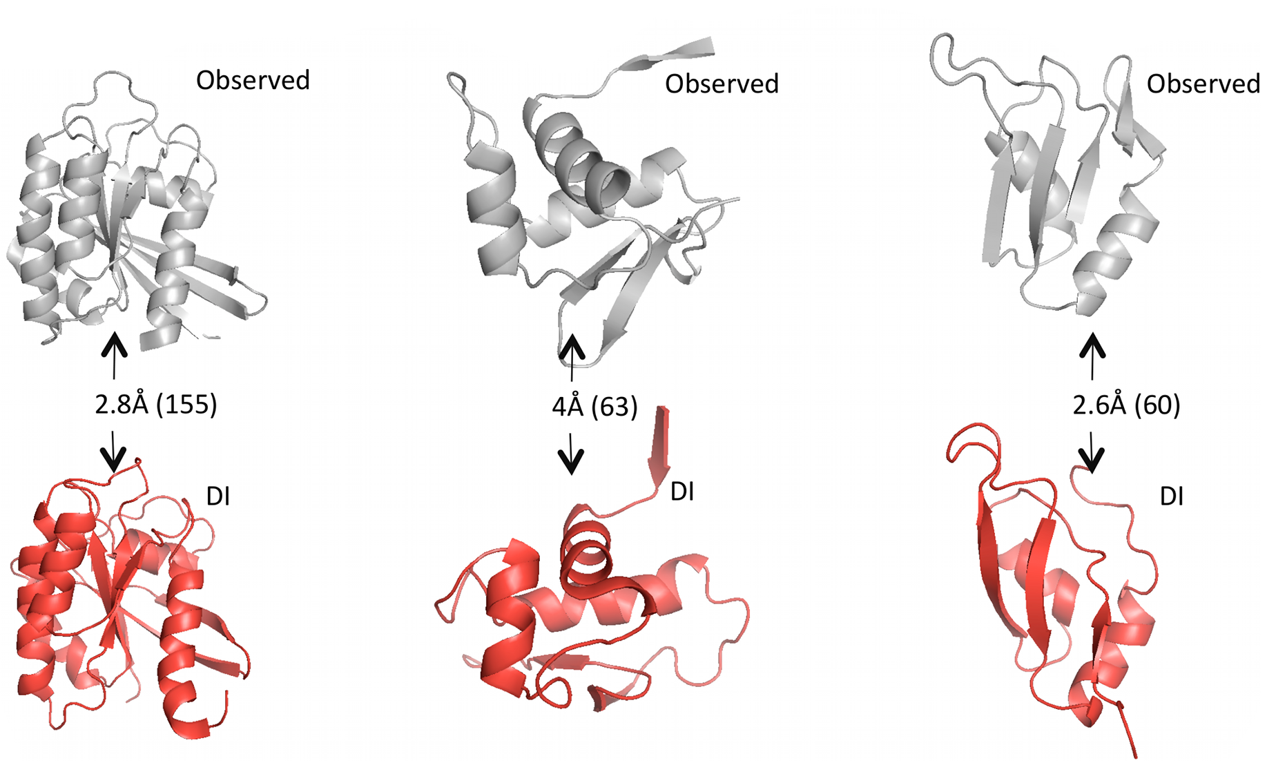
Grey structures are real, experimentally observed; red structures are predicted using DI. Root mean square deviation (RMSD) measures the average distance between atoms in the predicted vs. observed structure and is used to score the quality of structure predictions; they are shown on the arrows with the total number of amino acid positions in parentheses. Figure from 1.

Predicting function

At this point, you might think: this is all neat and all, but is it directly useful in any way? One common problem in industrial biotechnology is: given a protein that carries out some useful function – e.g. an enzyme that catalyses a desired reaction – how can we improve it by increasing its stability or activity?

One approach is saturation mutagenesis: take the protein's sequence, mutate every position to every possible amino acid, and test all the mutants to see if any yields an improvement. I know that sounds crazy, but it has been made possible by impressive developments in automation-enabled high-throughput screening (in comparison, progress in our biological understanding necessary to make more informed guesses has generally lagged behind). Can we do better?

Predicting mutation effects

Remember our energy function that measures the fitness of a sequence in the context of an MSA:

Intuitively, sequences with low energy should be more likely to fail. Perhaps we can let energy guide our experimental testing. Let $A^{\mathrm{wt}}$ be a wildtype, or natural, sequence, and let $A^{\mathrm{mut}}$ be a mutant sequence:

captures how much the mutant's energy improved over the wildtype.

In this paper introducing the mutation effect prediction tool in EVCouplings, researchers computed the $\Delta E$ of each mutant sequence in a saturation mutagenesis experiment on a protein called M.HaeIII 3.

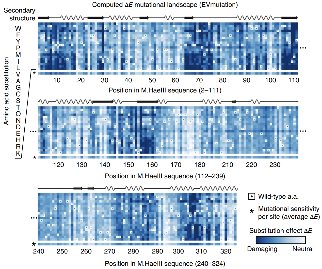
Deeper shades of blue reflect more negative ΔE. Most mutations are damaging. Averages across amino acids are shown as a bar on the bottom, labeled with * (sensitivity per site). Figure from 3.

Not all positions are created equal: mutations at some positions are especially harmful. The big swathes of blue (damaging mutations) speak to the difficulty of engineering proteins.

The calculated energies correlated strongly with experimentally observed fitness (!), meaning that our energy function provides helpful guidance on how a given mutation might affect function. It's remarkable that with such a simple model and from seemly so little information (just MSAs!), we can attain such profound predictive power.

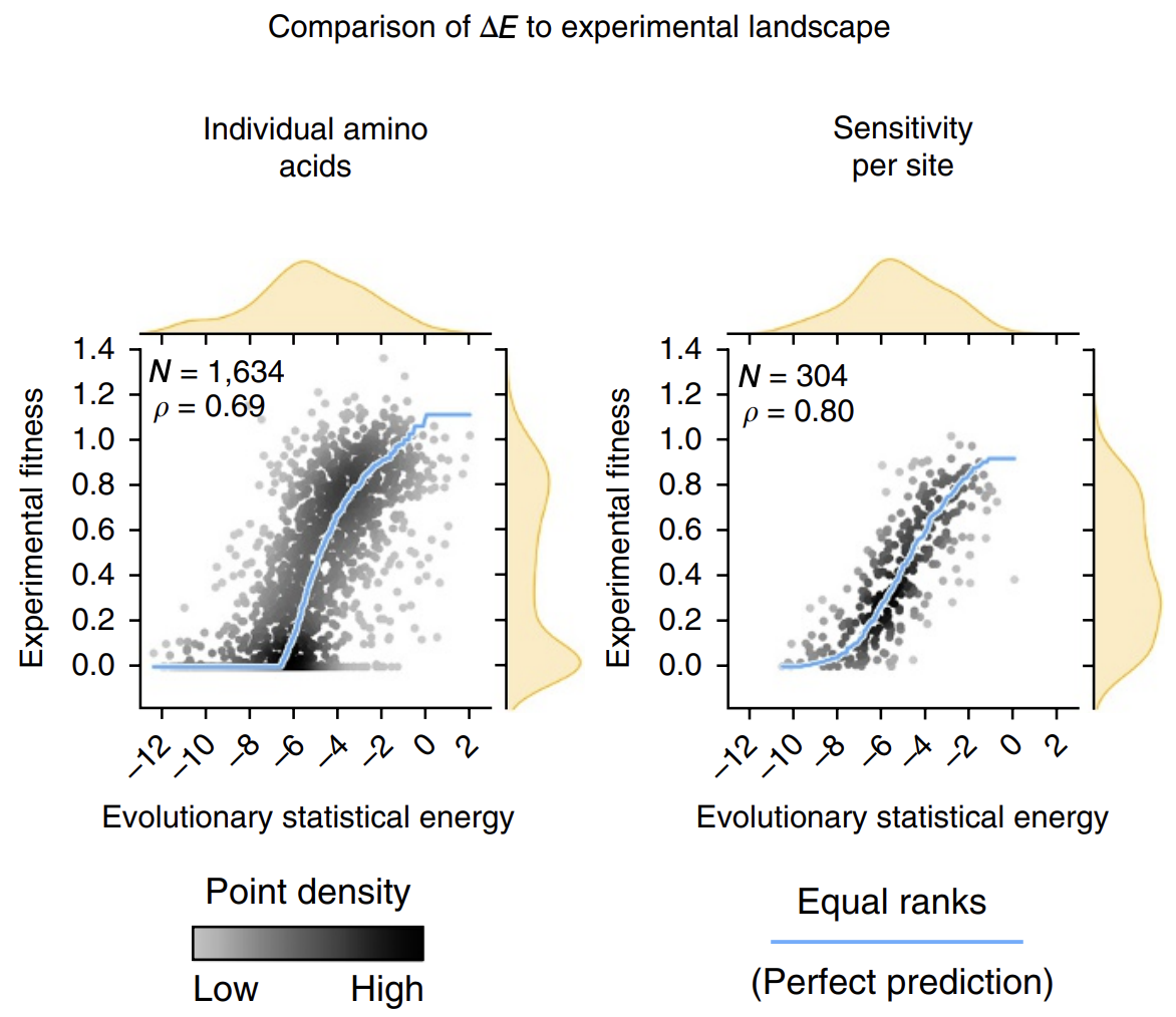
Evolutionary statistical energy refers to our energy function E. Left plot shows all mutants; right plot shows averages over amino acids at each position. Figure from 3.

The next time we find ourselves trying a saturation mutagenesis screen to identify an improved mutant, we can calculate some $\Delta E$'s first before stepping in the lab and can perhaps save time by focusing only on the sequences with more positive $\Delta E$'s that are more likely to work.

Generating new sequences

Only considering point mutations is kinda lame: what if the sequence we're differ at several positions from the original? To venture outside the vicinity of the original sequence, let's try this:

1. Start with a random sequence $A$.
2. Mutate a random position to create a candidate sequence $A^{\mathrm{cand}}$.
3. Compare $E(A)$ with $E(A^{\mathrm{cand}})$.
   • if energy increased, awesome: accept the candidate.
   • if energy decreased, still accept the candidate with some probability proportional the energy difference and ideally with a knob we can control, like $P_{\mathrm{accept}} = \exp(-\Delta E / T)$.
     • the bigger this $\Delta E$, which goes in the unwanted direction, the smaller the acceptance probability.
     • $T \in (0, 1]$ lets us control how forgiving we want to be: $T \to 1$ makes accepting more likely; $T \to 0$ makes accepting less likely. $T$ is called the temperature.
4. Go back to 2. and repeat many times.

In the end, we'll have a sequence that is a random sample from our probability distribution (slightly modified from before to include $T$).

Why this works involves a lot of cool math that we won't have time to dive into now. This is the Metropolis–Hastings algorithm, belonging to a class of useful tools for approximating complex distributions called Markov chain Monte Carlo (MCMC).

In this paper, researchers did exactly this to with the goal of improving a protein called chorismate mutase (CM) 4. They used MCMC to draw many sequences from the DCA distribution and then synthesized them for experimental testing.

When they set $T = 0.33$ (second row in the figure below), they created sequences with:

1. higher energy than natural sequences (the energy they use is the negative of our $E(A)$, i.e. the smaller the better)
2. enhanced activity compared to natural CM when expressed in E. coli (!)

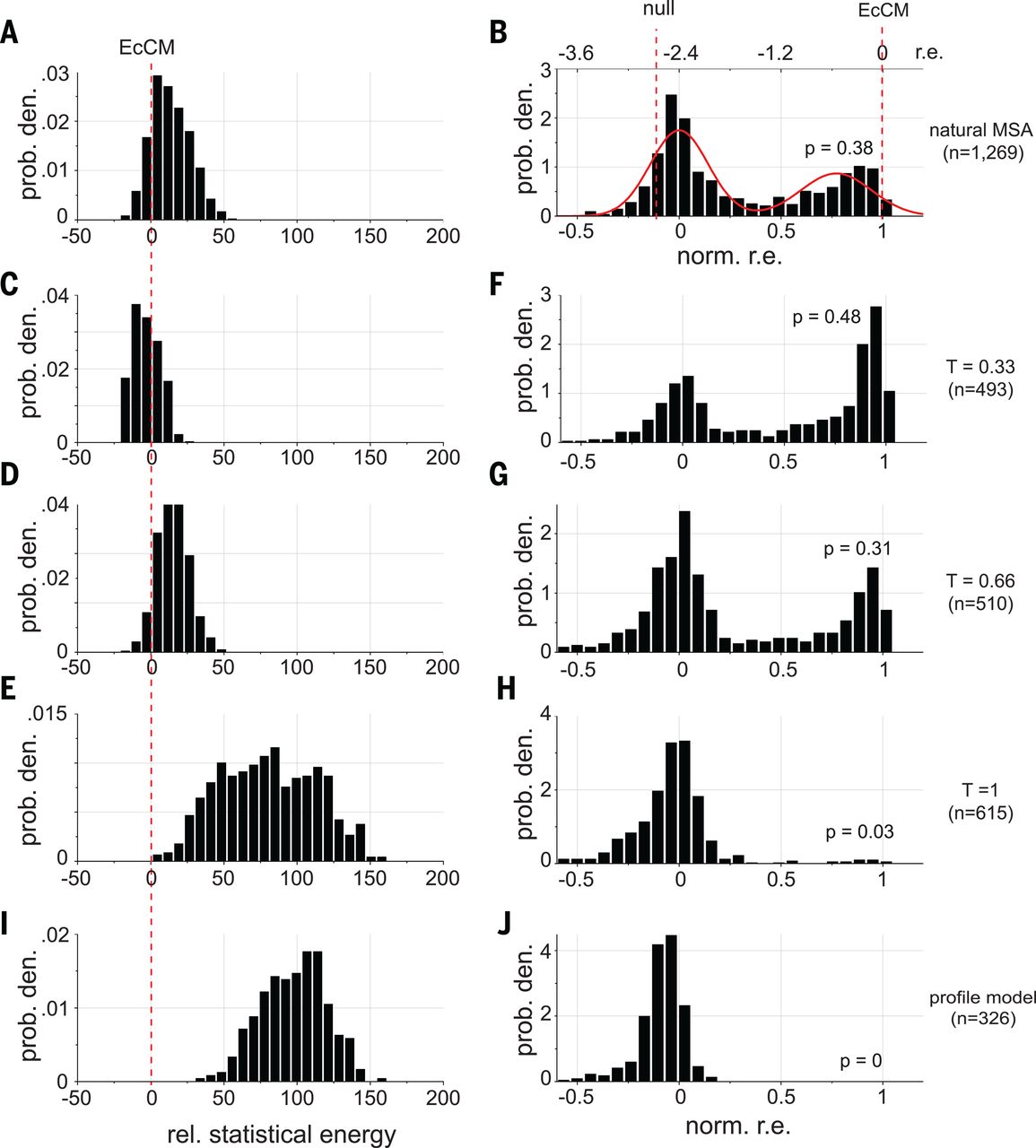
EcCM is a natural CM whose high activity is used as a benchmark and goalpost. Statistical energies on the left are negatives of ours, i.e. the smaller the better. norm. r.e. on the right stands for normalized relative enrichment; absent more experimental details, we can interpret them as: more density around norm r.e. = 1 means higher CM activity. At T = 0.33 (second row), we saw improvements in both statistical energy (left) and experimental CM activity (right) over natural proteins. The profile model on the bottom row contains only the independent h terms and no pairwise J terms, with expected poor performance. Figure from 4.

Taken together, a simple DCA model gave us the amazing ability to improve on the best that nature had to offer! Our energy function enables us to not only check a given sequence for its fitness, but also generate new ones with high fitness.

Summary + what's next

We talked about the direct coupling analysis (DCA) model with some of its cool applications. I hope by now you would join me in the fascination and appreciation of MSAs.

There are limitations: for example, DCA doesn't work well on rare sequences for which we lack the data to construct a deep MSA. Single-sequence methods like UniRep 9 and ESM 10 combat this problem (and come with their own tradeoffs). I will dive into them in a future post.

Recently, a deep learning mechanism called attention 5, the technology underlying magical large language models like GPT, has taken the world by storm. As it turns out, protein sequences are much like natural language sequences on which attention prevails: a variant of attention called axial attention 6 works really well on MSAs 7 8, giving rise to models with even better performance. I also hope to do a deep dive on this soon!

Links

The ideas we discussed are primarily based on:

• Protein 3D structure computed from evolutionary sequence variation focuses on 3D structure prediction, describes DCA in detail, and provides helpful intuitions. It's a highly accessible and worthwhile read.

• Mutation effects predicted from sequence co-variation presents the results on predicting mutation effects and introduces the powerful EVMutation.

• An evolution-based model for designing chorismate mutase enzymes is an end-to-end protein engineering case study using our model.

I also recommend the following papers that extend these ideas:

• Robust and accurate prediction of residue–residue interactions across protein interfaces using evolutionary information applies this model to protein-protein interfaces, for which we need the MSAs of the two proteins side by side.

• Evolutionary couplings detect side-chain interactions dives into some nuances and limitations of this approach: our structure prediction method using $J_{ij}$'s is mostly good at detecting interactions between side chains, and their orientations matter.

(In these papers and the literature in general, the word residue is usually used to refer to what we have called amino acid position. For example, "we tested a protein with 100 residues"; "we measured interresidue distances in the folded structure"; "residues in spatial proximity tend to co-evolve".)

References

Marks, D.S. et al. Protein 3D structure computed from evolutionary sequence variation. PLoS One 6, e28766 (2011).
Weigt, M et al. Direct-coupling analysis of residue coevolution captures native contacts across many protein families. Proc. Natl. Acad. Sci. (2011).
Hopf, T. et al. Mutation effects predicted from sequence co-variation. Nat Biotechnol 35, 128–135 (2017).
Russ W.P. et al. An evolution-based model for designing chorismate mutase enzymes. Science. 2020;369(6502):440–445 (2020).
Vaswani A. et al. Attention is all you need. NeurIPS (2017).
Ho J. et al. Axial Attention in Multidimensional Transformers. arXiv (2019).
Rao, R.M. et al. MSA Transformer. Proceedings of Machine Learning Research 139:8844-8856 (2021).
Jumper, J. et al. Highly accurate protein structure prediction with AlphaFold. Nature 596, 583–589 (2021).
Alley, E.C. et al. Unified rational protein engineering with sequence-based deep representation learning. Nat Methods 16, 1315–1322 (2019).
Rives, A. et al. Biological structure and function emerge from scaling unsupervised learning to 250 million protein sequences. Proc. Natl. Acad. Sci. (2021).