Protein Inception
October 9, 2023
Models that are good at making predictions also possess some generative power. We saw this theme play out in previous posts with a technique called Markov Chain Monte Carlo (MCMC). Here’s a quick recap:
Imagine you have a monkey that, when shown an image, gets visibly excited if the image contains bananas – and sad otherwise.
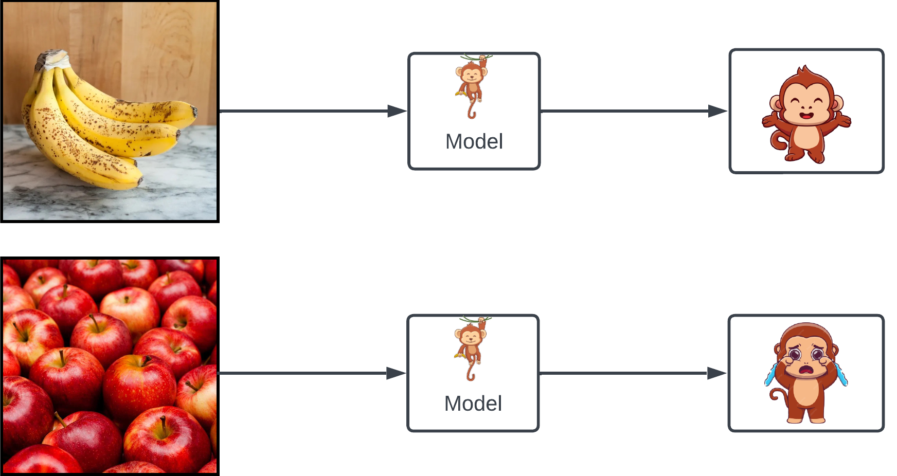
An obvious task the monkey can help with is image classification: discriminate images containing bananas from ones that don’t. The monkey is a discriminative model.
Now suppose you want to create some new images of bananas. We can start with a white-noise image:

randomly change a couple pixels, and show it to our monkey:
- If he gets more excited, then we’ve probably done something that made the image more banana-like. Great – let’s keep the changes.
- If he doesn’t get more excited – or God forbid, gets less excited – let’s discard the changes .
Repeat this thousands of times: we’ll end up with an image that looks a lot like bananas! This is the essence of MCMC, which turns our monkey into a generative model.
Researchers at Google used a similar technique in a cool project called DeepDream. Instead of monkeys, they used convolutional neural networks (CNNs).
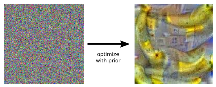
“Optimize with prior” refers to the fact that to make this work well, we usually need to constrain our generated images to have some features of natural images: for example, neighboring pixels should be correlated. Figure from and more details in this blog post on DeepDream.
The resulting images have a dream-like quality and are often called hallucinations.
Let’s replace the banana recognition task with one we’re not so good at: predicting the fitness of proteins – and creating new ones with desired properties. The ability to do this is revolutionary to industrial biotechnology and therapeutics. In this post, we’ll explore how approaches similar to DeepDream can be used to design new proteins.
The model: trRosetta
Overview
transform-restrained Rosetta (trRosetta) is a structure prediction model that, like almost everything we’ll talk about in this post, was developed at the Baker lab 1. trRosetta has 2 steps:
-
Given a Multiple Sequence Alignment (MSA), use a CNN to predict 6 structure-defining numbers for each pair of residues .
-
Use the 6 numbers produced by the CNN as input to the Rosetta structure modeling software to generate 3D structures.
Let’s focus on step 1. One structure-defining number produced by trRosetta is the distance between the residues, . There’s also this angle :
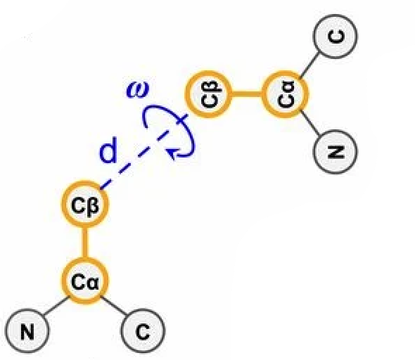
C (alpha-carbon), is the first carbon in the amino acid’s side chain; C (beta-carbon) is the second. Simplistically, imagine your index fingers as side chains: C’s are the bases of your fingers, C’s are the fingertips, and , the C-C distance, is the distance between your fingertips. Figure from 1.
as well as 4 other angles:
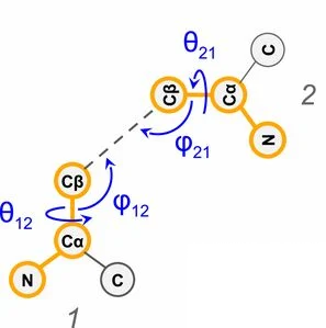
Figure from 1.
If we know these 6 numbers for each residue pair in folded 3D structure, then we should have a decent sense of what the structure looks like – a good foundation for step 2.
The architecture
Here’s the architecture of the trRosetta CNN. For our purposes, understanding the inner workings is not as important. The big picture: the network takes in an MSA and spits out these interresidue distances and orientation angles.
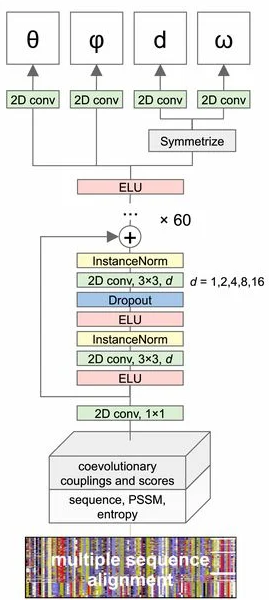
trRosetta uses a deep residual CNN. For more details, check out the trRosetta paper. Figure from 1.
Distance maps
Let’s ignore the angles for now and focus on distance. The interresidue distances predicted by the network are presented in a matrix called the distance map:
Surrounding the diagonal of the matrix are residues that are close in sequence position – which are of course close in 3D space – explaining the dark diagonal line. (Only the residues that are far apart in sequence but close in 3D are interesting and structure-defining.)
In this simplified visualization of an amino acid chain’s folded structure, the fact that residues 2 and 3 (close in sequence, on diagonal of matrix) are close in space is obvious and uninteresting, but the fact that 2 and 8 (far in sequence, off diagonal of matrix) are close in space – due to some interresidue interaction represented by the blue link – is important for structure.
Neural networks output probabilities. For example, language models like GPT – tasked with predicting the next word given some previous words as context – outputs a probability distribution over the set of all possible words (the vocabulary); in an additional final step, the word with the highest probability is chosen to be the prediction. In our case, trRosetta outputs probabilities for different distance bins, like this:
| Distance bin | Probability |
|---|---|
| 0 - 0.5 Å | 0.0001 |
| 0.5 - 1 Å | 0.0002 |
| … | … |
| 5 - 5.5 Å | 0.01 |
| 5.5 - 6.0Å | 0.74 |
| 6.0 - 6.5Å | 0.12 |
| … | … |
| 19.5 - 20 Å | 0 |
An angstrom (Å) is m, a common unit for measuring atomic distance. Each distance bin spans 5 Å and is assigned a probability by trRosetta.
In this example, it’s pretty clear that trRosetta believes the distance between these two residues to be around 6 Å, which we can use as our prediction. Because trRosetta is so confident, we say that the distance map is sharp.
But trRosetta is not always so confident. If the probability distribution is more uniform, it wouldn’t be so clear which distance bin is best. In those cases, we say the distance map is blurry.
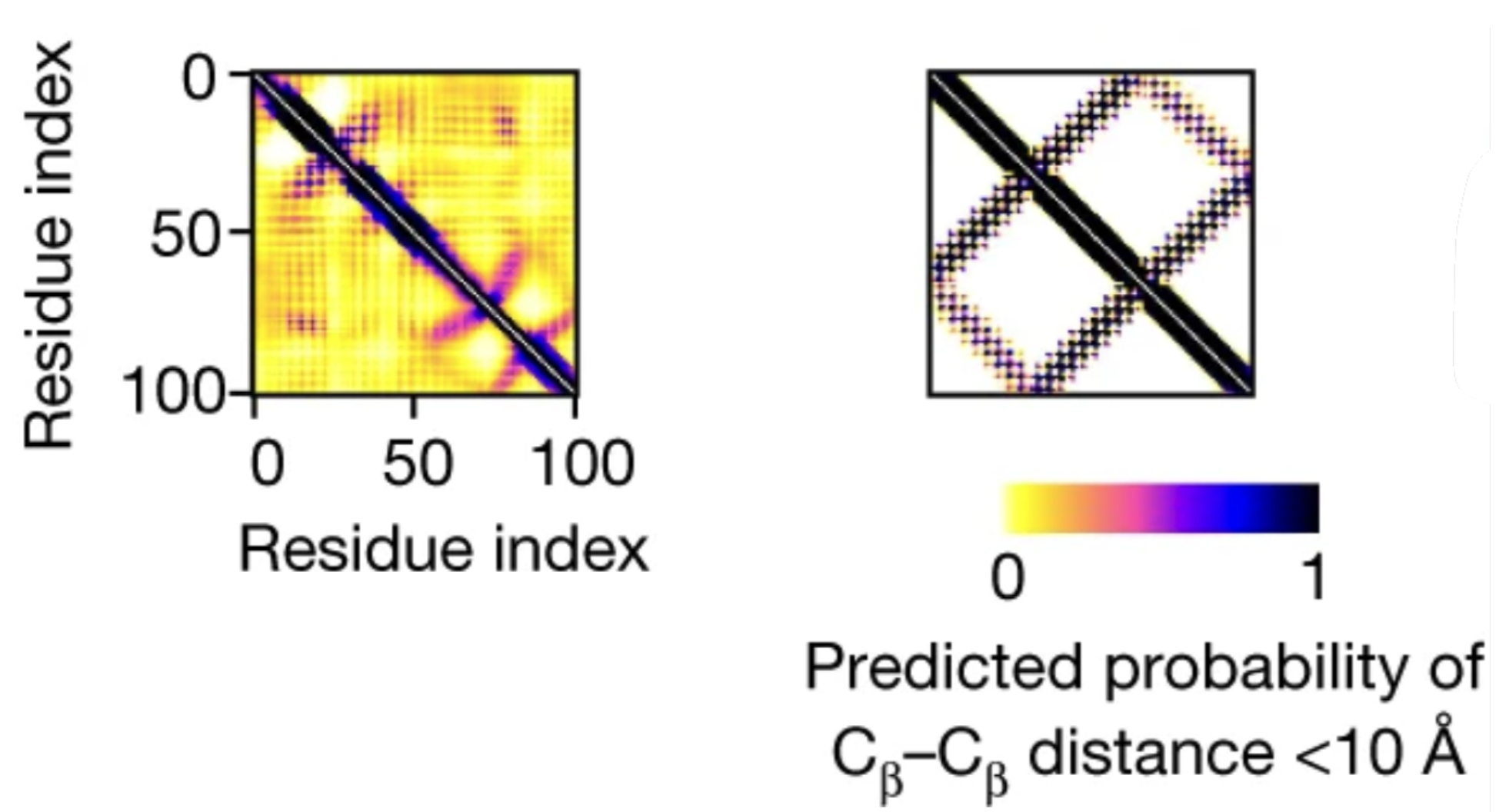
Let’s visualize this. In the two distance maps we showed above, the colors reflect, for each residue pair, the sum of trRosetta’s predicted probabilities for the bins in the range, i.e. how likely trRosetta thinks it is for the residues to end up close together in the 3D structure.
Figure from 2.
The left distance map is blurry, while the right one is sharp.
If we provide trRosetta a garbage sequence that doesn’t even encode a stable protein, no matter how good trRosetta is at its job of predicting distances, the distance map will be blurry; after all, how can trRosetta be sure if we ask for the impossible? Conversely, if we provide good sequences of stable proteins, trRosetta will produce sharp distance maps.
This idea is important because sharpness, like the monkey’s excitement for bananas, is a signal that we can rely on to discriminate good sequences from bad ones.
Quantifying sharpness
Leo Tolstoy famously said:
All happy families are alike; each unhappy family is unhappy in its own way.
For distances maps produced by trRosetta, it’s kinda the opposite: all blurry distance maps are alike; each sharp distance map is sharp in its own way. Each functional protein has a unique structure – that determines a specific function – something that trRosetta learns to capture, whereas each nonfunctional sequence is kinda the same to trRosetta: a whole lotta garbage.
Let’s quantify sharpness by coming up with a canonical blurry distance map – a bad example – to steer away from: a distance map is sharp if it’s very different from 2.
We can get from a background network, which is the same as trRosetta with one important catch: the identity of each residue is hidden in the training data. The background network retains some rudimentary information about the amino acid chain, e.g. residues that are close in sequence are close in space. But it cannot learn anything about the interactions between amino acids determined by their unique chemistries.
Given some distance map , how do we measure its similarity to our bad example, ? Remember, a distance map is just a collection of probability distributions, one for each residue pair. If we can measure the difference in the probability distributions at each position – vs. – we can average over those measurements and get a measurement between and :
where is the length of the sequence, measures similarity between distance maps, and measures similarity between probability distributions.
Here’s one way to measure the similarity between two distributions:
where is the predicted probability of the distance between the residues and falling into bin .
This is the Kullback–Leibler (KL) divergence, which came from information theory. It’s a common loss function in machine learning.
To summarize, we have developed a way to quantify the sharpness of a distance map :
is sharp if it’s as far away from as possible, as measured by the average KL divergence.
Hallucinating proteins
To recap, when fed an amino acid sequence that encodes a functional protein, trRosetta produces a sharp distance map, a good foundation for structure prediction.
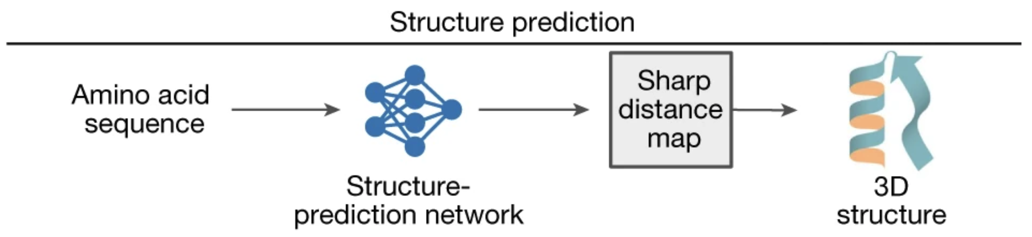
Figure from 2.
When fed a random amino acid sequence, trRosetta produces a blurry distance map. But, equipped with a tool to measure sharpness, we can sharpen the blurry distance map using MCMC 2.
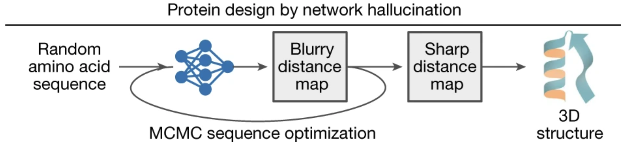
Figure from 2.
Let’s start with a random sequence analogous to a white-noise image. At each MCMC step:
- Make a random mutation in the sequence.
- Feed the sequence into trRosetta to produce a distance map .
- Compare to , the blurry distance map generated by hiding amino acid identities.
- Accept the mutation with high probability if it is a move in the right direction: maximizing the average KL divergence between and .
- this acceptance criterion is called the Metropolis criterion.
- an additional parameter, , is introduced as a knob we can use to control acceptance probability.
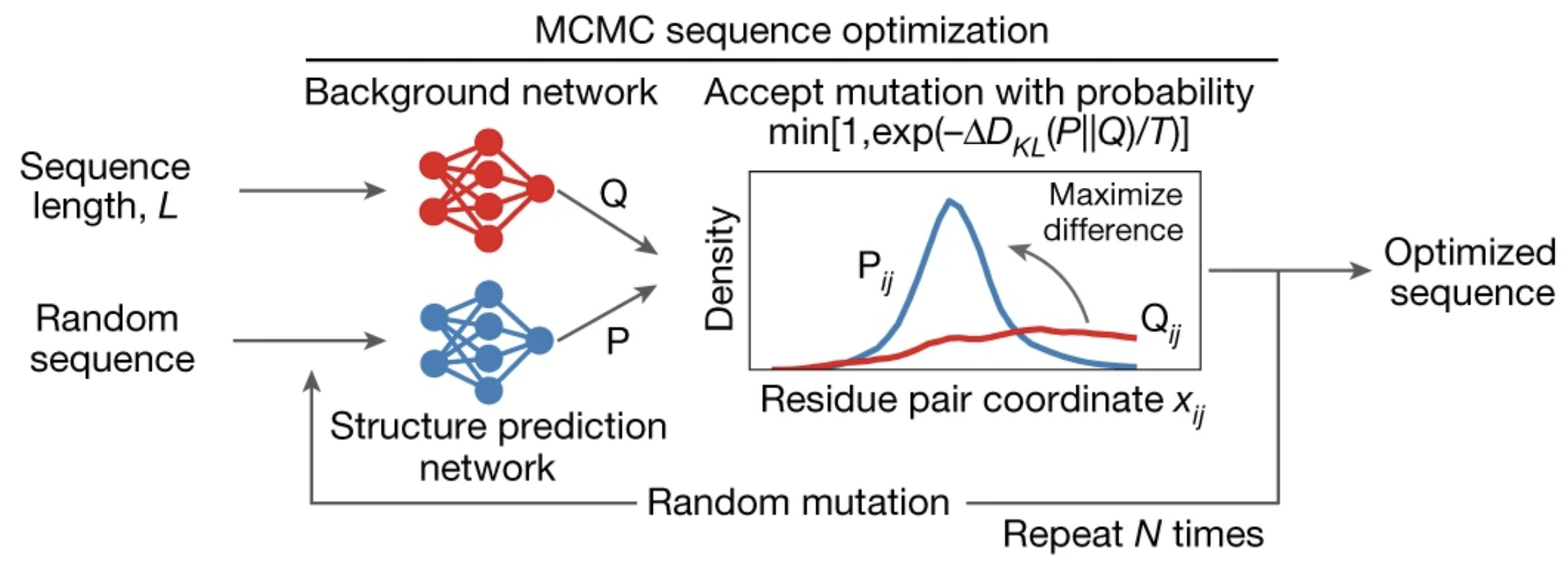
Figure from 2.
As we repeat these steps, the distance maps get progressively sharper, converging on a final, sharp distance map after 40,000 iterations.
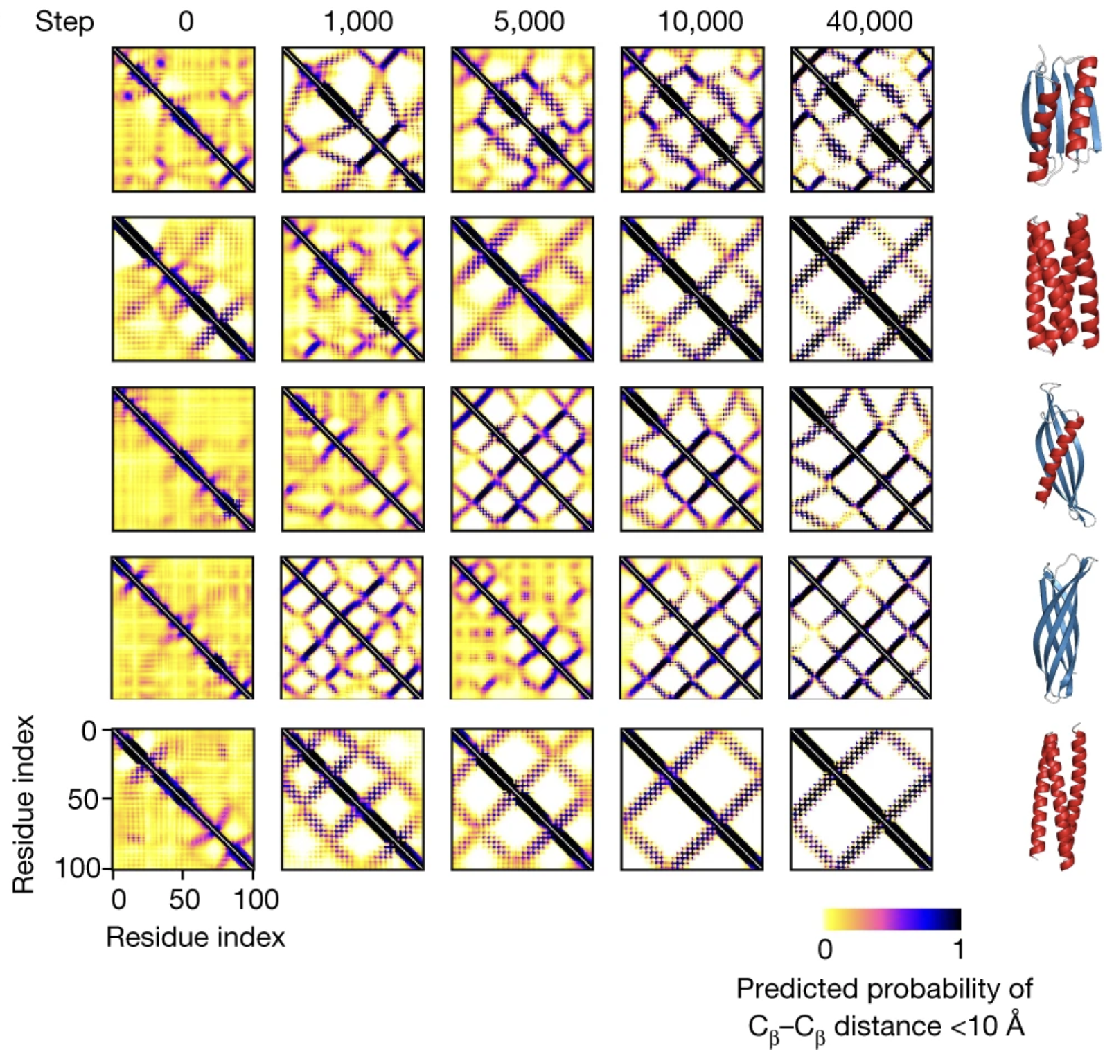
Each row represents a Monte Carlo trajectory, the evolutionary path from a random protein to a hallucinated protein. Distance maps get progressively sharper along the trajectory. Final predicted structures are shown on the right. Figure from 2.
When expressed in E. coli, many of these these hallucinated sequences fold into stable structures that closely match trRosetta’s predictions.
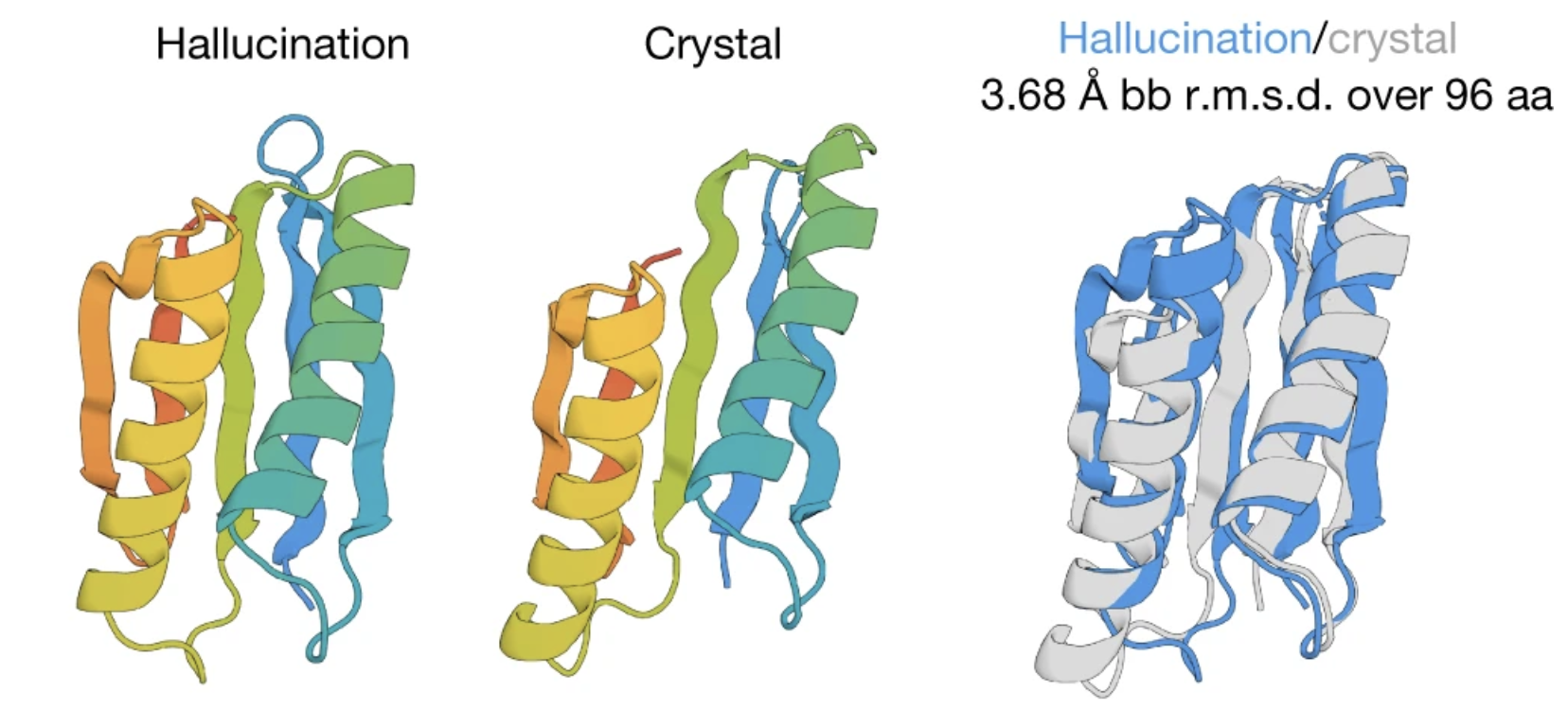
Here’s one of the hallucinated sequences. We compare trRosetta’s predicted structure to the experimental structure obtained via X-ray crystallography after expressing the sequence in E. coli. The ribbon diagram on the right shows the two overlaid on top of each other. Figure from 2.
I find this astonishing. We can create stable proteins that have never existed in nature, guided purely by some information that trRosetta has learned about what a protein should look like.
Can we do better than MCMC?
MCMC is fundamentally inefficient. We’re literally making random changes to see what sticks. Can we make more informed changes, perhaps using some directional hints from the knowledgeable trRosetta?
There’s just the thing in deep neural networks like trRosetta: gradients 3. During training, gradients guide trRosetta in adjusting its parameters to make better structure predictions .
We already have a loss function: our average KL divergence between and . At each step:
- Ask the differentiable trRosetta to compute gradients with respect to the loss.
- Use the gradients to propose a mutation instead of using a random one.
- Turning the gradients into a proposed mutation takes a few simple steps (bottom left of the diagram). They are explained in the methods section here.
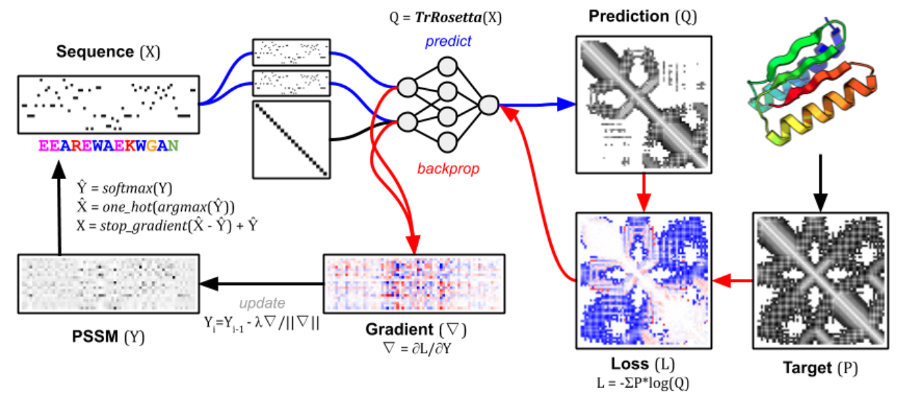
The figure describes a more constrained version of protein design called fixed-backbone design, which seeks an amino acid sequence given a target structure 3. This is why the loss function, in addition to the KL divergence term, also contains a term measuring similarity to the target structure (right). Nonetheless, the principles of leveraging gradients to create more informed mutations are the same, regardless of whether we have a target structure. Figure from 3.
Using this gradient-based approach, we can often converge to a sharp sequence map with much fewer steps, usually hundreds instead of tens of thousands.
Designing useful proteins
So far, we have focused on creating stable proteins that fold into well-predicted structures. Let’s take it one step further and design some proteins that have a desired function, such as binding to a therapeutically relevant target protein.
Functional sites
Most proteins perform their function via a functional site formed by a small subset of residues called a motif. For example, the functional sites of enzymes bind to their substrates and perform the catalytic function .
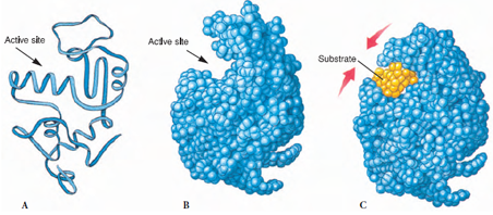
The functional sites of enzymes are called active sites. Figure from https://biocyclopedia.com/index/general_zoology/action_of_enzymes.php.
Since it’s really the functional site that matters, a natural problem is: given a desired functional site, can we design a protein that contains it? This is called scaffolding a functional site. Solutions to this problem has wide-ranging implications, from designing new vaccines to interfering with cancer 5.
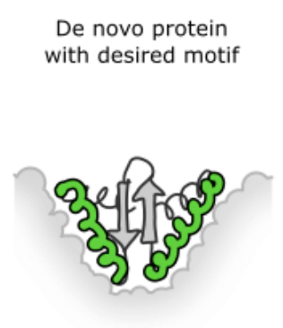
The green part is the motif we need; the grey part is what we need to design. Figure from 4.
Satisfying the motif
To guide MCMC towards sequences containing the desired motif, we can introduce an additional term to our loss function to capture motif satisfaction:
where , the free-hallucination loss, is our average DL divergence from before, nudging the model away from to be more generally protein-like; and is the new motif-satisfaction loss.
Intuitively, this loss needs to be small when the structure predicted by trRosetta clearly contains the desired motif – and big otherwise (for the mathematical details, check out the methods section here). We are engaging in a balancing act: we want proteins that contain the functional site (low motif-satisfaction loss) that are also generally good, stable proteins (low free-hallucination loss)!
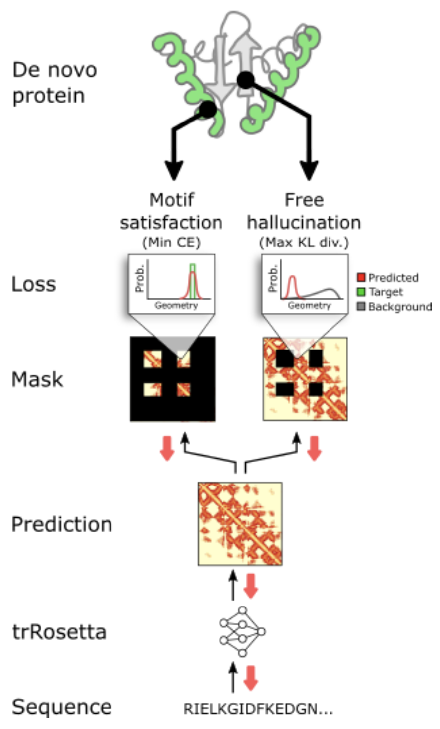
We take trRosetta’s predicted distance maps and look at them in two ways: 1. look at the residues that correspond to the motif: do they do a good job recreating the motif? (motif-satisfaction) ; 2. look at the rest of the residues: do they look protein-like? (free-hallucination). Figure from 4.
A case study: SARS-CoV-2
SARS-CoV-2, the virus behind the Covid-19 pandemic, has a clever way of entering our cells. It takes advantage of an innocent, blood-pressure regulating protein in our body called angiotensin-converting enzyme 2 (ACE2) attached to the cell membrane.
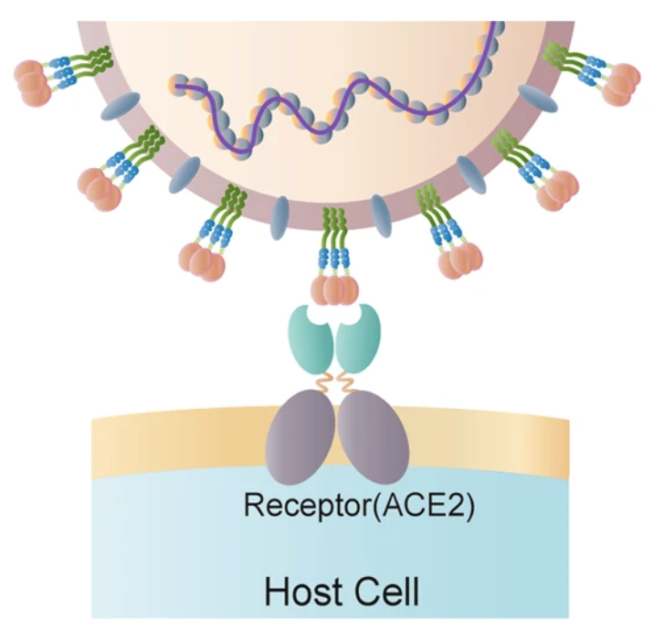
ACE2 on the cell membrane. The coronavirus contains spike proteins that bind to ACE2. Figure from 6.
It anchors itself by binding to an alpha helix in ACE2, and then enters the cell:
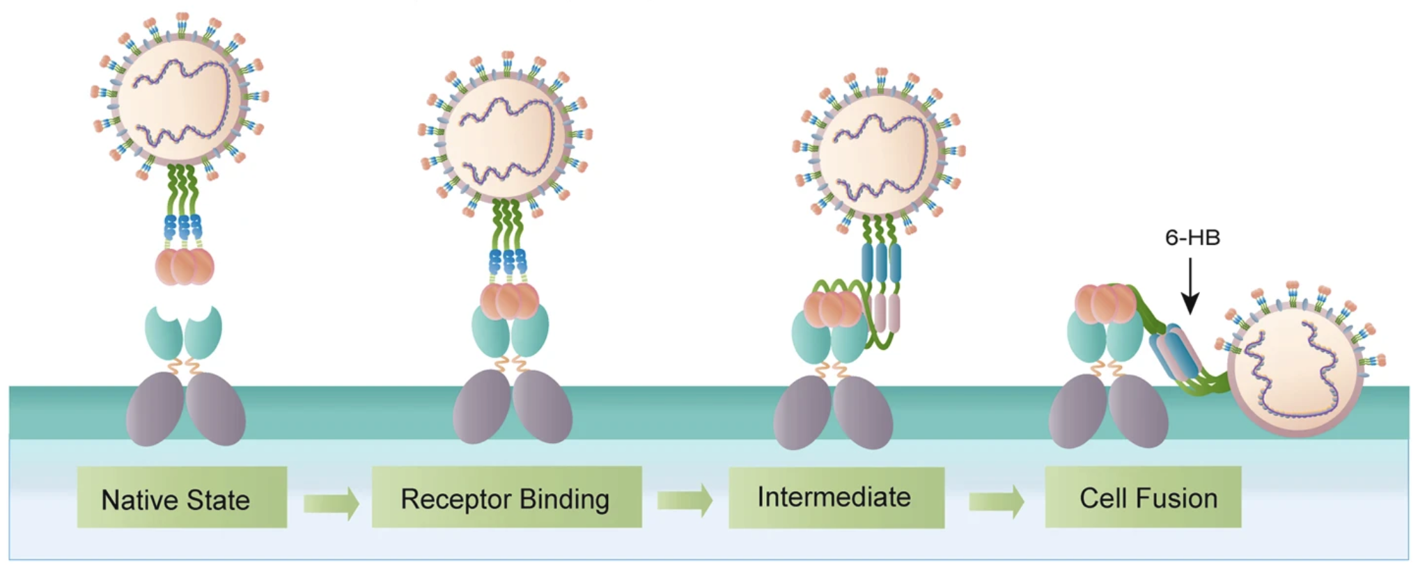
The coronavirus takes advantage of ACE2 to enter the cell and eventually dumps its viral DNA into the cell :( Figure from 6.
One way we can disrupt this mechanism is to design a protein that contains ACE2’s interface alpha helix. Our protein would trick the coronavirus into thinking that it is ACE2 and bind to it, sparing our innocent ACE2’s. These therapeutic proteins are called receptor traps: they trap the receptors on the coronavirus spike protein.
This is exactly our functional site scaffolding problem. Folks at the Baker lab used the composite loss function to hallucinated these receptor traps containing the interface helix (shown on the right).
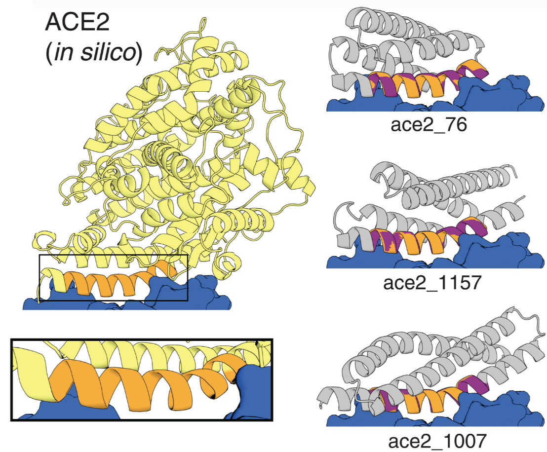
Light yellow: Native protein scaffold of ACE2. Grey: hallucinated scaffolds. Orange: the interface helix (our target motif). Blue: spike proteins that binds to the helix. Figure from 5.
I hope I have convinced you that these hallucinations are not only cool but also profoundly useful. And of course, this is only the tip of the iceberg: the ability to engineer proteins that disrupt disease mechanisms will revolutionize drug discovery and reduce a lot of suffering in the world.
Final notes
-
Throughout this post, we exclusively focused on the distances produced by trRosetta, represented in distance maps. There are also the 5 angles parameters that work in the exact same way: binned predictions, KL divergence, etc. trRosetta outputs 1 distance map and 5 “angle”-maps, all of which are used to drive the hallucinations.
-
trRosetta is no longer the best structure prediction model, a testament to this rapidly moving field. Since 2021, two models have consistently demonstrated superior performance: AlphaFold from DeepMind and RoseTTAFold from the Baker lab.
- Both AlphaFold and RoseTTAFold are deep neural networks, so all the ideas discussed in this post still apply.
- This paper applies the same techniques using AlphaFold; many subsequent papers from the Baker lab use RoseTTAFold instead of trRosetta, including the one that designed the SARS-CoV-2 receptor trap 5.
-
Have I mentioned the Baker lab yet? If you are new to all this, check out David Baker’s TED talk on power of designing proteins.
Acknowledgements
Thank you to Jue Wang for reading drafts of this post and giving feedback.
References
Yang, J. et al. Improved protein structure prediction using predicted interresidue orientations. Proc. Natl. Acad. Sci. (2021).
Anishchenko, I. et al. De novo protein design by deep network hallucination. Nature 600, 547–552 (2021).
Anishchenko, I. et al. Protein sequence design by conformational landscape optimization. Proc. Natl. Acad. Sci. (2021).
Tischer, D. et al Design of proteins presenting discontinuous functional sites using deep learning. arXiv (2020).
Wang, J. et al Scaffolding protein functional sites using deep learning. Science 377,387-394 (2022).
Huang, Y. et al. Structural and functional properties of SARS-CoV-2 spike protein. Acta Pharmacol Sin 41, 1141–1149 (2020).
- In Metropolis-Hastings, we still accept this change some percentage of the time, proportional to how counterproductive it was.
- Residue, meaning unit, refers to a position in the amino acid chain.
- Notation is slightly rewritten to be consistent with this paper. It's conventional to use double bars like to emphasize the fact that , i.e. KL divergence is not a distance metric.
- If you're new to deep learning, I highly recommend this video by Andrej Karpathy explaining gradients from the ground up.
- Enzymes are proteins that catalyze a reaction by binding to the reactant, called substrate. Enzyme are indispensible to our bodily functions: as you read this, an enzyme called PDE6 catalyzes the reactions converting the light hitting your retina to signals sent to your brain.
- We left out an important detail: how do we choose which residues should constitute the motif? The cited paper tried two approaches, described in a section called 'Motif placement algorithms'.